RC Time Constant Calculator
Calculate RC time constant plus charging or discharging voltage, current, charge, and stored energy at a selected time.
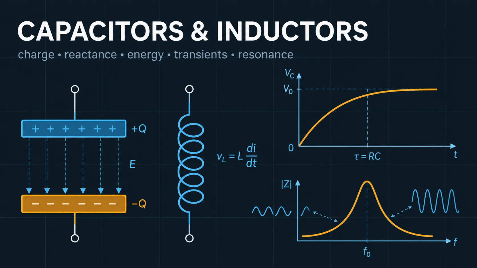
Learn electric and magnetic energy storage through capacitor and inductor networks, physical geometry, dielectrics, transients, reactance, coupling, and LC resonance.
These standalone calculators use calculation engines from this workbench and provide direct, focused pages for common engineering checks.
Calculate RC time constant plus charging or discharging voltage, current, charge, and stored energy at a selected time.
Calculate capacitor charge and stored energy from capacitance and voltage.
Calculate inductive reactance, RMS current, reactive power, angular frequency, and peak flux linkage.