Atomic Structure & Diffusion Workbench

Interactive workspace initializes in your browser. Engineering method, assumptions, validation, and references are available below.

Engineering reference

Atomic Structure & Diffusion: theory, method, and sources

This materials science workspace publishes 9 governing equations, 5 stated assumptions, 1 documented boundary, 2 worked examples, 1 validation case, and 3 sources so the numbers it returns can be checked rather than taken on trust.

Calculations run locallyContent reviewed September 8, 2026Calculation & source methodology

How this tool works

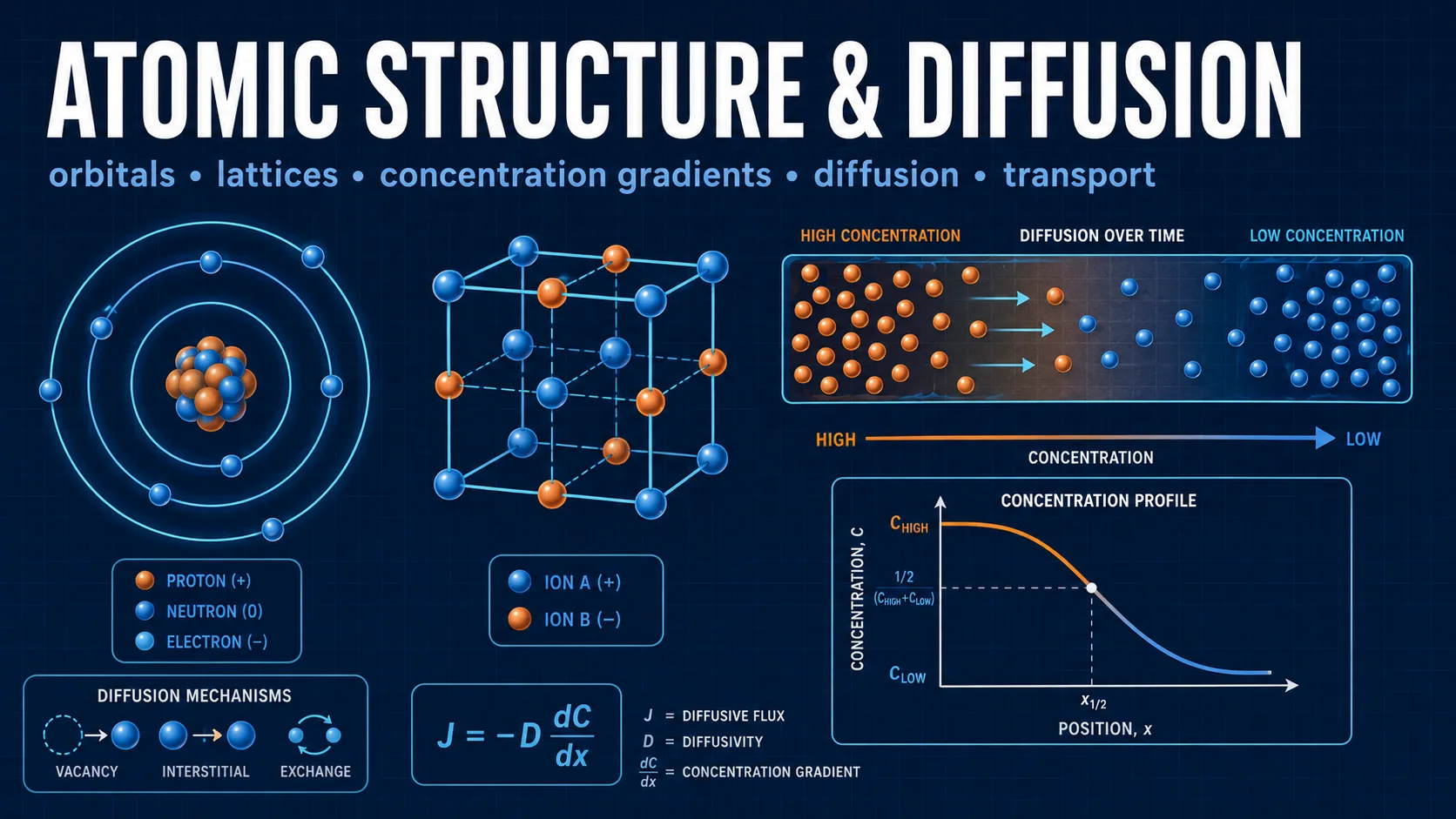
Ten modules cover unit cell density, cubic packing factors, Miller indices, interplanar spacing, Bragg diffraction, vacancy concentration, Arrhenius diffusivity, Fick flux, diffusion length, and the rule of mixtures for alloy density.

Use the Arrhenius module to calculate diffusivity, then enter that diffusivity in the independent flux or diffusion-length module. Values are not transferred automatically between these modules.

Engineering theory

Reciprocal intercepts define a plane

Miller indices describe the orientation of a lattice plane using integer ratios. Express each intercept in units of its corresponding lattice parameter, take the reciprocals, and multiply all three by the same factor until a reduced integer triple is obtained. Preserve a negative intercept as a negative index. Independently rounding the three reciprocals changes their ratio and can describe a different plane.

This calculator accepts three finite, nonzero intercepts. It searches for a common scale up to index magnitude 10000 and rejects ratios it cannot resolve at its numerical tolerance. An axis-parallel plane has an infinite intercept and zero corresponding index; that case is outside this finite-intercept entry form. A plane through the origin requires choosing a parallel representative before taking reciprocals.

Mass fractions and volume fractions are different inputs

The alloy-density calculator takes weight fractions, normalizes their sum, and assumes additive constituent volumes. For a chosen total mass, each constituent occupies its mass divided by its density. Add these volumes and divide the total mass by the total volume. This gives the inverse density rule, not the arithmetic density average used for volume fractions. Porosity, reaction, and volume change on mixing can invalidate this ideal estimate.

Diffusion length describes a root-mean-square displacement under a constant diffusion coefficient. Select one, two, or three spatial dimensions explicitly. It is not the maximum distance reached by an atom or a sharp interface in a heat-treated material. Temperature changes, grain boundaries, and composition-dependent diffusion require a richer model.

Inputs and outputs explained

Inputs

Plane interceptslattice-parameter multiples: Enter signed rational intercepts. Values such as 1, 5, and 7 represent distances along the corresponding crystal axes.
Mixture fractionsmass fraction: Enter nonnegative weight fractions with matching positive densities. The calculator normalizes the fractions; percentages and fractions therefore give the same composition.

Outputs

Miller indices: The smallest integer ratio resolved from the reciprocal intercepts, with signs preserved.
Mixture densitykg/m³: Total mass divided by total constituent volume under the stated volume-additivity assumption.

Calculators and topics covered

crystallography
diffusion
XRD
defects
unit cells
Miller indices
Bragg law
Fick law
vacancy concentration
diffusivity

Core equations

\text{unit cell density:}\quad \rho = \frac{nA}{V_{c}\; N_{A}}

\text{atomic packing factor:}\quad SC = 0.52,\; BCC = 0.68,\; FCC = 0.74

\text{cubic interplanar spacing:}\quad d = \frac{a}{\sqrt{h^{2} + k^{2} + l^{2}}}

\text{Bragg law:}\quad n\lambda = 2 d\; \sin \; \theta

\text{vacancy fraction:}\quad \frac{N_{v}}{N} = \exp \left(\frac{- Q_{v}}{kT}\right)

\text{Arrhenius diffusivity:}\quad D = D_{0} \exp \left(\frac{- Q}{kT}\right)

\text{Fick’s first law:}\quad J = - D \left(\frac{\Delta C}{\Delta x}\right)

\text{RMS diffusion distance:}\quad x_{rms} = \sqrt{2\; n_{\mathrm{dim}}\; D\; t}

\text{density from weight fractions:}\quad \begin{gathered}\frac{1}{\rho } = \sum \left(\frac{w_{i}}{\rho _{i}}\right)\\\sum w_{i} = 1\end{gathered}

Worked examples

Plane with intercepts 1, 5, and 7

A plane intercepts its crystal axes at 1a, 5b, and 7c.

Method

Take reciprocals: 1, 1/5, and 1/7.
Multiply every reciprocal by 35: 35, 7, and 5.
The integers have no common factor greater than one.

Result: Miller indices are (35 7 5).

Interpretation: A fixed rounding grid could incorrectly return (6 1 1). Reconstructing the reciprocal ratio makes that error visible.

Equal constituent masses

Mix equal masses of constituents with densities 8000 and 2000 kg/m³, assuming additive volumes.

Method

Choose total mass 1 kg: each constituent has mass 0.5 kg.
Total volume is 0.5/8000 + 0.5/2000 = 0.0003125 m³.
Divide 1 kg by this volume.

Result: Mixture density is 3200 kg/m³.

Interpretation: The lower-density constituent occupies more volume. The arithmetic average, 5000 kg/m³, corresponds to equal volumes and is incorrect for these mass inputs.

Common mistakes

Confusing fraction basis

Using the arithmetic density average with weight fractions.

Better approach: Use the inverse rule for mass fractions; use the arithmetic rule only for volume fractions under additive-volume assumptions.

Method and assumptions

Assumptions

Crystals are treated as perfect and defect-free apart from the vacancy concentration explicitly calculated.
Diffusivity follows a single Arrhenius relationship over the temperature range, with no change in mechanism.
Fick’s first law assumes steady state with a linear concentration gradient.
Diffusion length is a characteristic scale, not a sharp boundary; the full error-function solution is not evaluated.
Grain boundary and dislocation short-circuit diffusion paths are not modelled separately from bulk diffusion.

Limitations and design boundaries

Educational screening models only. Material certification, process qualification, applicable standards, statistical variability, environmental conditioning, and professional engineering judgment are required for real selection or design.

Validation cases

These checks document how representative calculations are cross-checked against analytic or reference results.

Validation policy

Rational plane recovery

Analytic cross-check

Method: Recover the independently reduced reciprocal ratio for integer and fractional intercepts.
Expected: (1,5,7) → (35,7,5); (0.5,0.75,1.25) → (15,10,6).

Sources and references

Primary sources are preferred for ratings, standards, manufacturer data, and externally defined constants.

Source policy

University of Cambridge DoITPoMS: Lattice planes and Miller indicesReciprocal intercepts and integer plane indices.
Callister and Rethwisch, Materials Science and Engineering: An Introduction
Askeland and Wright, The Science and Engineering of Materials