Acids, Bases, and Equilibrium Learning Lab
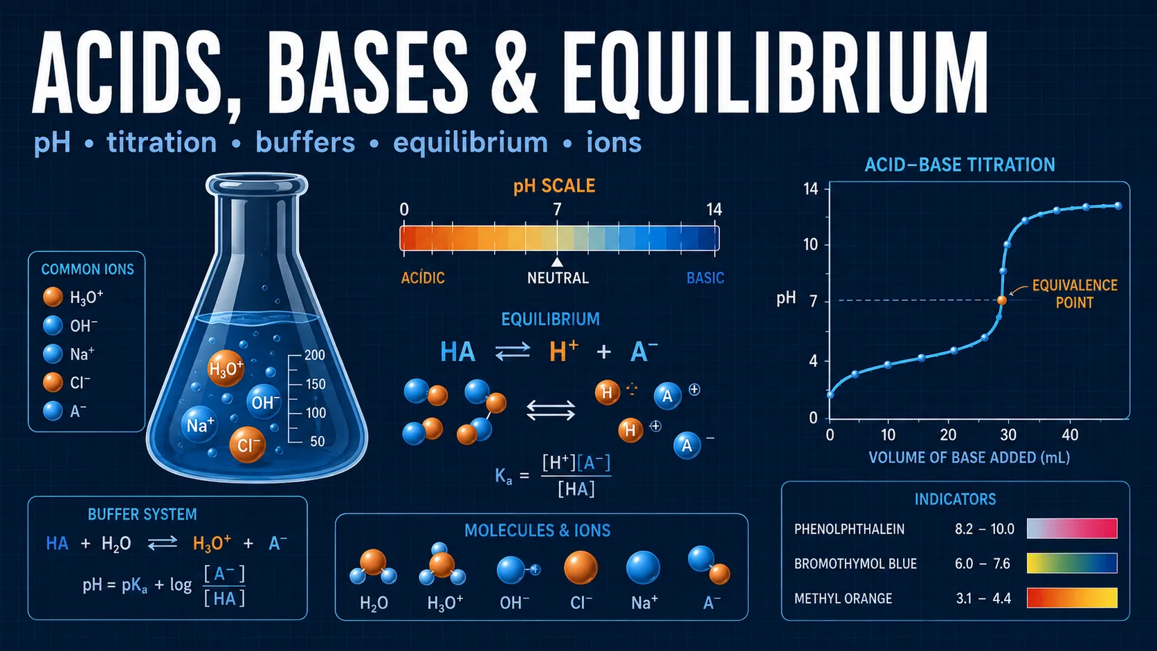
Fourteen guided chemistry lessons that connect particles, reactions, equations, graphs, and worked reasoning for acids, bases, equilibrium, buffers, titrations, and solubility.
Engineering reference
Acids, Bases & Equilibrium: theory, method, and sources
This chemistry workspace publishes 7 governing equations, 6 stated assumptions, 3 documented boundaries, and 3 sources so the numbers it returns can be checked rather than taken on trust.
How this tool works
The learning lab organizes fourteen acid–base and equilibrium topics into a five-unit sequence with explicit learning goals, real chemical contexts, guided observations, and live calculations.
Each lesson explains what the model represents, why the result changes, and how the current values connect to particle-level chemistry and laboratory reasoning.
Every numerical value, imported state, solver iteration, and graph sample count is bounded before calculation or rendering.
Calculators and topics covered
- acid base chemistry
- pH
- buffers
- titration
- chemical equilibrium
- ICE table
- Le Chatelier
- Ksp
- solubility
- pH calculator
- weak acid calculator
- weak base calculator
- buffer calculator
- Henderson Hasselbalch calculator
Core equations
Method and assumptions
Assumptions
- Aqueous acid–base calculations use Kw = 1.0×10⁻¹⁴ and pKw = 14.00 at 25 °C.
- Weak-acid and weak-base calculations use monoprotic ideal-solution models unless the polyprotic module is selected.
- Activity coefficients are approximated as one, so concentration is used in place of activity.
- Titration models assume additive volumes and complete stoichiometric neutralization by the strong titrant.
- Generic equilibrium modules model one homogeneous reaction of the form aA + bB ⇌ cC + dD.
- Kc–Kp conversion assumes ideal gases.
Limitations and design boundaries
- Highly concentrated solutions, mixed polyprotic systems, activity corrections, simultaneous equilibria, electrochemical equilibria, and full speciation with charge balance are outside this version.
- The Le Châtelier module predicts a new ideal equilibrium from one selected disturbance; it is not a kinetic simulation.
- Results are educational estimates and do not replace laboratory procedures, calibrated analytical software, or chemical safety review.
Sources and references
Primary sources are preferred for ratings, standards, manufacturer data, and externally defined constants.
- Harris, Quantitative Chemical AnalysisAcid and base equilibria, buffer behaviour, and titration curve construction.
- Skoog, West, Holler and Crouch, Fundamentals of Analytical ChemistryEquilibrium constant conventions, activity effects, and indicator selection.
- IUPAC Compendium of Chemical TerminologyDefinitions for pH, pKa, conjugate pairs, and standard state conventions.