Orbital Mechanics Simulator | Neutron STEM Lab

Loading interactive tool…

Engineering reference

Theory, method, validation, and sources

The interactive workspace is paired with its published engineering context: core equations, assumptions, design boundaries, and source references. Worked examples, validation cases, and editorial review dates are displayed only where that supporting evidence has been published for the tool.

Calculations run locallyContent reviewed August 10, 2026Calculation & source methodology

How this tool works

Propagate spacecraft trajectories with a bounded fourth-order Runge–Kutta integrator using ideal two-body gravity and an optional first-order J2 acceleration term.

Initialize the spacecraft from classical orbital elements or Cartesian position/velocity, then convert between representations and inspect the resulting osculating elements.

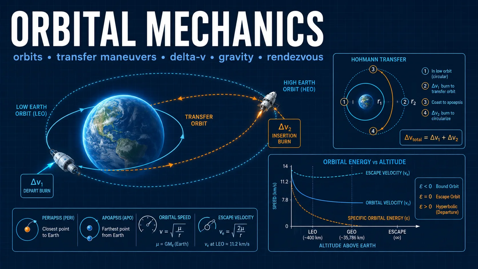
Apply one impulsive maneuver in the local radial/transverse/normal frame, preview circular-to-circular Hohmann transfers, animate the propagated path, rotate the 3D-style view, and scrub through time.

Engineering theory

A state vector and orbital elements describe the same two-body orbit

Cartesian position and velocity are convenient for numerical propagation and maneuvers, while classical elements describe the conic geometry and its orientation. The simulator converts both representations so a user can inspect how a burn changes semi-major axis, eccentricity, inclination, node, periapsis orientation, and anomaly.

Circular and equatorial orbits contain geometric singularities in the classical element definitions. In those cases the simulator uses stable fallback angle conventions rather than implying that an undefined node or periapsis direction has unique physical meaning.

Impulsive burns are evaluated in the local RTN frame

The radial axis points away from the central body, the transverse axis lies in the instantaneous orbital plane in the direction of motion, and the normal axis is parallel to orbital angular momentum. This makes prograde/retrograde, radial, and plane-changing components easier to reason about than inertial XYZ velocity changes.

A real thruster burns over finite time and changes spacecraft mass. The instantaneous RTN impulse is therefore a mission-design approximation, not a propulsion execution model.

Numerical propagation should be checked for convergence

The simulator uses bounded fixed-step RK4. If the trajectory changes materially when the time step is reduced, the coarse result is not numerically converged. The two-body mode reports specific-mechanical-energy drift as one useful numerical diagnostic.

J2 changes the conservative potential, so the simple two-body energy diagnostic is intentionally disabled when J2 propagation is active.

Inputs and outputs explained

Inputs

Central body: Preset Sun/planet/moon or custom gravitational parameter, radius, and optional J2 coefficient.
Classical elementskm, degrees: Semi-major axis, eccentricity, inclination, RAAN, argument of periapsis, and true anomaly.
Cartesian state vectorkm, km/s: Inertial position and velocity components relative to the central body.
Propagation durationhours: Requested trajectory duration.
Integration steps: Requested fixed RK4 step. Very long runs are automatically bounded to a finite number of output intervals.
RTN burnm/s: Optional radial, transverse, and normal impulsive velocity change at a selected simulation time.

Outputs

Trajectory: Time history of inertial position and velocity plus derived altitude and speed.
Osculating elements: Classical elements derived from the propagated final Cartesian state.
Altitude envelopekm: Minimum and maximum radius above the modeled body surface.
Peak speedkm/s: Maximum propagated inertial speed.
Energy drift: Relative change in two-body specific mechanical energy for runs without J2 or an impulse.
Hohmann preview: First/second burn, total Δv, and half-ellipse transfer time for circular-to-circular transfer planning.

Calculators and topics covered

orbital mechanics
orbit simulator
astrodynamics
spacecraft trajectory
Hohmann transfer
maneuver
state vector
orbital elements
free orbital mechanics simulator
online orbit simulator
spacecraft orbit propagation
classical orbital elements
impulsive burn
RTN burn

Core equations

r¨ = −μr/r³v² = μ(2/r − 1/a)p = a(1 − e²)r = p/(1 + e cosν)T = 2π√(a³/μ)Δv_RTN = ΔvR r̂ + ΔvT t̂ + ΔvN n̂aJ2 ∝ (3/2)J2 μR²/r⁵

Worked examples

400 km Earth orbit

Start near a 400 km circular Earth orbit with a 51.6° inclination and propagate slightly more than one revolution.

Inputs

a ≈ 6778.137 km
e = 0
i = 51.6°
J2 off

Result: The trajectory closes after about 92.6 minutes and the altitude remains approximately constant in the ideal two-body model.

Interpretation: Reducing the integration step should make the specific-energy drift approach zero.

LEO to GEO Hohmann transfer

Start from a circular 400 km Earth orbit and target a 35,786 km circular altitude.

Result: The preview produces the two ideal coplanar burns and transfer time; loading the transfer scenario applies the first prograde burn and propagates to the opposite apsis.

Interpretation: The second circularization burn is reported but not automatically applied in the first-release single-burn propagator.

Common mistakes

Entering altitude as semi-major axis

Classical semi-major axis is measured from the central-body center, not from its surface.

Better approach: For a circular Earth orbit at altitude h, use a = R_Earth + h.

Treating RTN and XYZ as the same frame

A transverse burn is defined relative to the instantaneous orbit, not the inertial X or Y axis.

Better approach: Use the RTN labels when reasoning about prograde/retrograde, radial, or normal maneuver components.

Using a large step because the path still looks smooth

A smooth rendered polyline can hide integration error.

Better approach: Repeat the run with a smaller step and compare the final state or energy-drift diagnostic.

Reading a J2 run as a complete perturbation model

J2 is only one perturbation and does not include drag, third bodies, radiation pressure, tesseral harmonics, or real ephemerides.

Better approach: Use dedicated astrodynamics software for operational orbit prediction.

Method and assumptions

Convert the selected initial representation into an inertial Cartesian state.

Integrate r¨ = a(r) with fixed-step RK4. If enabled, add the selected body J2 acceleration.

At the requested maneuver time, construct the local RTN basis from position and angular momentum and apply the instantaneous Δv.

Derive final osculating elements, trajectory extrema, impact state, and numerical diagnostics from the propagated history.

Assumptions

The propagation frame is central-body-centered and inertial; the central body itself is fixed at the origin.
The base model uses point-mass two-body gravity. Optional J2 adds only the standard first-order oblateness acceleration for the selected body constant.
Impulsive burns change velocity instantaneously in the local RTN frame and do not model finite thrust, propellant depletion, attitude dynamics, or execution uncertainty.
Hohmann guidance assumes coplanar circular initial and final orbits around the same central body.
Preset body constants are fixed educational reference values rather than time-dependent ephemerides.

Limitations and design boundaries

This is an educational and preliminary mission-design simulator, not an operational flight-dynamics, navigation, conjunction-assessment, or maneuver-certification tool.
The first release does not include atmospheric drag, third-body gravity, solar radiation pressure, finite burns, low-thrust propagation, Lambert targeting, real ephemerides, covariance propagation, collision avoidance, or n-body integration.
The canvas uses an orthographic 3D projection for visualization. Apparent screen distances are not a perspective camera measurement.
Very long or stiff trajectories require dedicated astrodynamics software and validated numerical methods.

Validation cases

These checks document how representative calculations are cross-checked against analytic or reference results.

Validation policy

Circular Earth orbit period

Analytic cross-check

Method: Convert a = Earth radius + 400 km, e = 0 to Cartesian state and evaluate T = 2π√(a³/μ).
Expected: Approximately 92.56 minutes.
Tolerance: Within numerical rounding of the fixed Earth μ and radius used by the tool.

Elements ↔ state round trip

Verified result

Method: Convert a non-singular elliptical orbit to Cartesian state and back to classical elements.
Expected: Semi-major axis, eccentricity, inclination, RAAN, argument of periapsis, and true anomaly return within floating-point tolerance.

Two-body energy conservation