Pipe Flow Calculators: Reynolds Number, Head Loss & Sizing

Interactive workspace initializes in your browser. Engineering method, assumptions, validation, and references are available below.

Engineering reference

Internal Pipe Flow: theory, method, and sources

This fluid mechanics workspace publishes 10 governing equations, 5 stated assumptions, 1 documented boundary, 1 worked example, and 2 sources so the numbers it returns can be checked rather than taken on trust.

Calculations run locallyContent reviewed August 11, 2026Calculation & source methodology

How this tool works

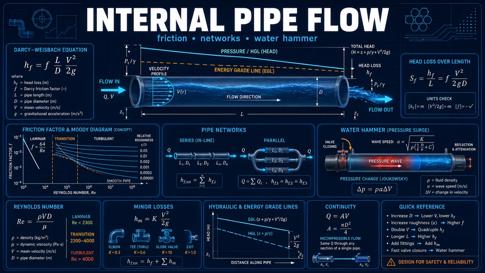
Eleven modules cover continuity, Reynolds number and flow regime, friction factor, major and minor losses, laminar Hagen–Poiseuille flow, equivalent length, water hammer, series and parallel pipe networks, and pipe sizing.

The network and sizing modules solve numerically by bisection, so a diameter or branch flow can be found directly from an allowable head loss instead of being iterated by hand.

Calculators and topics covered

pipes
friction
head loss
water hammer
Darcy-Weisbach
Reynolds number
Moody chart
minor losses
Hagen-Poiseuille

Core equations

\text{continuity:}\quad Q = AV\; \text{with}\; A = \frac{\pi D^{2}}{4}

\text{Reynolds number:}\quad \mathrm{Re} = \frac{\rho VD}{\mu }\; \left(\text{laminar}\; \text{below}\; 2300,\; \text{turbulent}\; \text{above}\; 4000\right)

\text{laminar friction factor:}\quad f = \frac{64}{\mathrm{Re}}

\text{Swamee–Jain turbulent friction factor:}\quad f = \frac{0.25}{\left[log_{10} \left(\frac{\varepsilon }{3.7 D} \frac{+ 5.74}{\mathrm{Re}^{0.9}}\right)\right]^{2}}

\text{Darcy–Weisbach:}\quad h_{f} = \frac{f \left(\frac{L}{D}\right) V^{2}}{2 g},\; \Delta p = \rho g \cdot h_{f}

\text{minor losses:}\quad h_{m} = \frac{\sum K \cdot V^{2}}{2 g}

\text{Hagen–Poiseuille:}\quad Q = \frac{\pi D^{4} \Delta p}{128 \mu L}

\text{equivalent length:}\quad L_{e} = \frac{KD}{f}

\text{Joukowsky water hammer:}\quad \Delta p = \rho \cdot a \cdot \Delta v

\text{series pipes:}\quad \begin{gathered}h_{\mathrm{total}} = \sum h_{i}\\\text{parallel pipes:}\quad \text{equal}\; \text{head}\; \text{loss},\; \text{summed}\; \text{flow}\end{gathered}

Worked examples

Pressure drop in a 100 m DN100 water main

A pump delivers 0.02 m³/s of water at 20 °C through 100 m of DN100 commercial steel pipe. The run includes fittings totalling ΣK = 4.2. The question is the total head the pump must overcome, and how much of it comes from the fittings rather than the pipe.

Inputs

Q = 0.02 m³/s, D = 0.100 m, L = 100 m
Water at 20 °C: ρ = 998.2 kg/m³, µ = 1.002 × 10⁻³ Pa·s
Commercial steel roughness ε = 4.5 × 10⁻⁵ m, fittings ΣK = 4.2

Method

Flow area is A = πD²/4 = 7.854 × 10⁻³ m², so the mean velocity is V = Q/A = 2.546 m/s.
Reynolds number is Re = ρVD/µ = 2.537 × 10⁵, which is firmly turbulent and well above the 4000 threshold.
Relative roughness is ε/D = 4.5 × 10⁻⁴. The Swamee–Jain correlation gives a friction factor f = 0.018275.
Major loss follows Darcy–Weisbach: h_f = f(L/D)V²/(2g) = 6.042 m, equivalent to 59.15 kPa.
Minor losses are h_m = ΣK·V²/(2g) = 1.389 m.
Total head loss is 6.042 + 1.389 = 7.431 m, or about 72.8 kPa.

Result: The pump must overcome 7.431 m of head, of which 6.042 m is pipe friction and 1.389 m is fittings.

Interpretation: The fittings contribute 19% of the total, which is too large to neglect and a common source of undersized pumps on short runs. The proportion scales with L: halve the pipe length and the fittings become roughly a third of the loss. A useful sanity check is that the 2.55 m/s velocity sits inside the usual 1–3 m/s design band for water in steel — much above that and erosion and noise become the governing limits rather than pressure drop. Note the Swamee–Jain friction factor approximates the implicit Colebrook equation to within about 1% over this range of Re and ε/D.

Method and assumptions

Assumptions

Flow is steady, incompressible, and fully developed, with the pipe running full.
The Swamee–Jain correlation approximates the Colebrook equation and is accurate to roughly 1% over the usual range of relative roughness and Reynolds number.
Loss coefficients K are user-supplied and must match the fitting type and diameter.
The Joukowsky equation gives the maximum surge for instantaneous valve closure and overestimates the pressure rise for slower closure.
Pipe wall elasticity, entrained air, thermal effects, and non-Newtonian behaviour are not modelled.

Limitations and design boundaries

Educational screening calculations only. Real systems require verified fluid properties, calibrated coefficients, uncertainty analysis, applicable codes and standards, and qualified engineering review.

Sources and references

Primary sources are preferred for ratings, standards, manufacturer data, and externally defined constants.

Source policy

Çengel and Cimbala, Fluid Mechanics: Fundamentals and Applications
Munson et al., Fundamentals of Fluid Mechanics

Focused calculator routes

Quick calculations from this workbench

These standalone calculators use calculation engines from this workbench and provide direct, focused pages for common engineering checks.

Browse all calculators →

Reynolds Number Calculator

Calculate Reynolds number and classify internal pipe flow as laminar, transitional, or turbulent from fluid and pipe conditions.

Darcy–Weisbach Pressure Loss Calculator

Calculate pipe velocity, Reynolds number, Darcy friction factor, head loss, and pressure loss from volumetric flow.