How this tool works
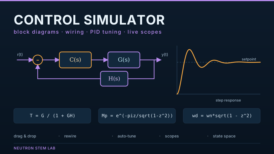
The simulator is a focused browser-based block-diagram environment for control-system learning and preliminary design. Add source, controller, plant, nonlinear, and scope blocks; wire them together; then simulate the complete closed loop instead of evaluating each equation in isolation.
It is free to use, requires no account or installation, and performs its interactive calculations in the browser. That makes it suitable for quick coursework, demonstrations, and control experiments on a shared or temporary computer.
Phase 2 UX is complete with a viewport-responsive diagram canvas, anchored zoom, Space/middle-mouse panning, fit-to-diagram, box and multi-selection, grouped block dragging, searchable drag-and-drop blocks, direct port wiring and drag-to-rewire, selectable/deletable wires, snap-to-grid, alignment/distribution tools, copy/paste/duplicate, and undo/redo history.
Included templates cover continuous PID/PI tracking, disturbance rejection, transfer functions, state-space plants, delay/noise and rate limits, plus Phase 3 sampled-data examples with digital PID, zero-order hold, discrete G(z), difference equations, discrete state space, and one-sample computation delay. Every template remains fully editable.
Scopes can be assigned as Reference, Output, Error, Control effort, or Auxiliary. When Reference and Output scopes exist, the simulator automatically calculates rise time, peak time, overshoot, settling time, steady-state error, IAE, ISE, ITAE, and ITSE.
The selected continuous or discrete PID block can be adjusted with live tuning sliders, ±10% gain nudges, optional auto-run, one-click rerun, gain revert, or numerical optimization. The first tuning change can preserve the current response as a baseline. Results use a sticky tabbed dock for overview, response, control, error, auxiliary, and linear analysis; time-domain scopes support cursor readouts, drag-to-zoom, Ctrl+wheel zoom, and synchronized time-window reset. Continuous linear-compatible feedback diagrams also derive closed-loop poles, reference-to-output frequency response, open-loop Bode response, bandwidth, gain margin, and phase margin.
Method and assumptions
The runtime converts supported continuous dynamic blocks into state derivatives, evaluates the connected diagram, and advances continuous states with classical fourth-order Runge–Kutta. Discrete blocks update at their sample events and retain outputs between events.
Performance metrics are derived from the simulated reference/output/error signals after a run. Linear analysis is constructed only when the diagram can be represented as the supported continuous small-signal model; otherwise it is explicitly withheld.
Assumptions
- Continuous dynamic blocks are simulated with a user-selected fixed base time step using RK4; digital blocks update only at their configured sample instants and hold outputs between updates.
- General transfer-function blocks must be strictly proper in this release so feedback diagrams do not require an algebraic-loop solver.
- Unconnected input ports evaluate to zero and are reported as warnings before simulation.
- PID derivative action uses a first-order derivative filter rather than an ideal differentiator.
- Automatic PID optimization is a local numerical search for the current diagram and test input; it is not a universal tuning guarantee.
- Digital sample times must be integer multiples of the fixed base simulation step in this release so mixed continuous/discrete event timing is deterministic.
- Linear analysis is a zero-operating-point continuous-time small-signal model. It is disabled when sampled-data blocks are present rather than presenting misleading continuous Bode margins for a digital loop.