Loading tool…
Loading interactive tool…

Engineering reference

Theory, method, validation, and sources

The interactive workspace is paired with its published engineering context: core equations, assumptions, design boundaries, and source references. Worked examples, validation cases, and editorial review dates are displayed only where that supporting evidence has been published for the tool.

Calculations run locallyContent reviewed August 11, 2026Calculation & source methodology

How this tool works

Nineteen modules cover the core undergraduate control-systems workflow, from first- and second-order transient response through classical frequency-domain design, state-space analysis, and discrete-time stability.

Charts are selected to match the engineering quantity being studied: pole, root-locus, Nyquist, and z-plane modules use complex-plane plots; Bode and margin modules use logarithmic frequency axes; time-response modules use time histories; modules without a meaningful chart report results directly instead of forcing unrelated quantities into a graph.

The PI module evaluates the actual PI-controlled first-order transfer function, including the controller zero, rather than substituting a standard second-order numerator.

Calculators and topics covered

  • control systems
  • feedback
  • stability
  • PID
  • root locus
  • Bode
  • Nyquist
  • state space
  • digital control
  • step response
  • time constant
  • damping ratio
  • natural frequency
  • overshoot

Core equations

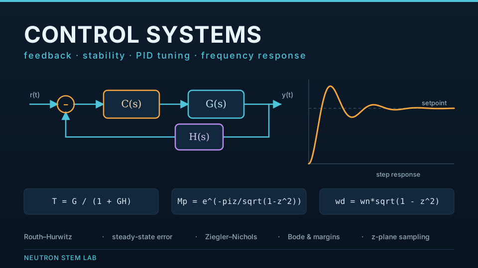
first-order lag: G(s)=K/(τs+1), y(t)=KU(1−e^(−t/τ))second-order form: G(s)=ωₙ²/(s²+2ζωₙs+ωₙ²)pole-zero model: G(s)=K(s+z)/(s²+a₁s+a₀)negative feedback: T=G/(1+GH), S=1/(1+GH)Routh criterion: first-column sign changes equal the number of right-half-plane rootssteady-state error: e_ss=A/(1+Kp), A/Kv, or A/Ka for step, ramp, or parabola inputsroot-locus example: 1+K/[s(s+a)(s+b)]=0Ziegler–Nichols PID: Kp=0.6Ku, Ti=Tu/2, Td=Tu/8PI closed loop: T(s)=KpK(Ti s+1)/[τTi s²+Ti(1+KpK)s+KpK]lead/lag: C(s)=K(1+sTz)/(1+sTp)first-order Bode: |G|=K/√(1+(ωτ)²), ∠G=−atan(ωτ)margins: GM=1/|L(jωpc)|, PM=180°+∠L(jωgc)state space: ẋ=Ax+Bu, y=Cx; controllability=[B AB], observability=[C;CA]canonical state feedback: K=[ωₙ²−a₀, 2ζωₙ−a₁]sampling: z=e^(sT), fN=fs/2discrete first order: y[k+1]=a y[k]+b u[k]second-order Jury conditions: |a₀|<1, 1+a₁+a₀>0, 1−a₁+a₀>0

Worked examples

PI control of a first-order thermal plant

A heater behaves as a first-order plant with a DC gain of 2 °C per unit of controller output and a time constant of 4 s. Open loop it takes about 12 s to reach 95% of a setpoint change and always leaves a steady-state offset. A PI controller is added to remove the offset and speed the loop up.

Inputs
  • Plant: K = 2, τ = 4 s, so G(s) = 2/(4s + 1)
  • Controller: K_p = 8, T_i = 0.2 s
  • Unit step setpoint change
Method
  1. The loop gain is K_p·K = 16. Closing a PI loop on a first-order plant gives the second-order characteristic polynomial τT_i s² + T_i(1 + K_pK)s + K_pK.
  2. That maps onto the standard form with ωₙ = √(K_pK/(τT_i)) = 4.472 rad/s and ζ = 0.4752.
  3. Because ζ < 1 the response is underdamped, with a damped frequency of ω_d = ωₙ√(1 − ζ²) = 3.935 rad/s.
  4. Overshoot follows M_p = exp(−πζ/√(1 − ζ²)) = 18.33%, peaking at t_p = π/ω_d = 0.798 s.
  5. The 2% settling time is approximately 4/(ζωₙ) = 1.882 s.
  6. The integrator drives steady-state error to zero for a step, so the loop settles exactly on the setpoint.

Result: The PI loop settles within 2% in 1.88 s with 18.3% overshoot and no steady-state offset, against roughly 12 s and a permanent offset for the plant alone.

Interpretation: The offset is gone because the integrator adds a pole at the origin, making this a type 1 loop. The 18.3% overshoot is the price of the aggressive integral time; lengthening T_i to 0.3 s at the same K_p raises ζ to 0.582 and cuts overshoot to 10.6% while leaving the settling time essentially unchanged at 1.88 s, which is usually the better trade for a thermal process. Note this treatment ignores actuator saturation — a real heater cannot deliver negative power, so a loop tuned this tightly will integrator-wind-up on a large setpoint step unless anti-windup is implemented.

Method and assumptions

Assumptions

  • Models are linear and time invariant unless a module explicitly describes a sampled recursion; actuator saturation, dead zones, backlash, quantisation, and rate limits are not represented.
  • Time-response calculations assume zero initial conditions and ideal step inputs.
  • The Routh module accepts real polynomials up to eighth order and handles a zero pivot with an epsilon substitution and a complete zero row with the auxiliary-polynomial derivative method.
  • The root-locus module uses the specific unity-feedback open-loop model K/[s(s+a)(s+b)] so the plotted branches have an unambiguous physical interpretation.
  • The lead/lag and Bode modules evaluate ideal rational transfer functions without transport delay.
  • Gain/phase margins and the Nyquist module use L(s)=K/[s(τ₁s+1)(τ₂s+1)].
  • The state-space controllability and observability module is restricted to a two-state SISO model.
  • State-feedback pole placement uses controllable canonical form; arbitrary A and B matrices require a general pole-placement algorithm.
  • Digital modules assume uniform periodic sampling and ideal arithmetic.

Limitations and design boundaries

  • This workbench is intended for teaching and preliminary analysis, not final safety-critical controller validation.
  • MIMO loop-shaping, observers/Kalman filters, LQR/LQG, H-infinity synthesis, nonlinear control, adaptive control, and model-predictive control are not yet implemented.
  • The Nyquist module focuses on a representative stable-plant loop form and does not automatically count arbitrary open-loop right-half-plane poles.
  • Controller tuning must still be validated against actuator limits, sensor noise, plant uncertainty, delays, and operating-point changes.
  • Numerical plots use finite sweeps and double-precision arithmetic; they are not substitutes for a dedicated simulation environment when high-order or stiff models are involved.

Sources and references

Primary sources are preferred for ratings, standards, manufacturer data, and externally defined constants.

Source policy
  • Ogata, Modern Control EngineeringTransient response, Routh–Hurwitz stability, root locus, state-space analysis, and pole placement.
  • Nise, Control Systems EngineeringPole-zero interpretation, steady-state error, frequency response, gain/phase margins, and compensator design.
  • Franklin, Powell and Emami-Naeini, Feedback Control of Dynamic SystemsSensitivity, state-space control, digital control, and frequency-domain design.
  • Åström and Murray, Feedback SystemsFeedback principles, robustness, loop shaping, state-space models, and digital implementation.
  • Åström and Hägglund, PID Controllers: Theory, Design, and TuningPID structure, practical tuning, and limitations of Ziegler–Nichols rules.